Forecasting Stock Prices Using Recurrent Neural Networks

Machine learning (ML) has taken gargantuan steps in every field imaginable. From smart cars to detecting brain tumours¹, it has infiltrated every field, leaving in its wake, a new era – the augmented era. I like to think of it as a time when man and “machine” work together for optimal output. The most notable of this is the design industry where 3D printed structures are now designed by ML algorithms to increase structural integrity while reducing material consumption². Most empirical sciences have readily welcomed this with open arms. Econometrics, finances, credit risk analysis, and game theory are some fields of economics where ML influence is strongly visible. In the course of this article, I wish to show you a working deep learning model that forecasts (predicts, if you will) the prices of a particular stock.

Perhaps a brief introduction to the world of artificial intelligence (AI) is due, particularly for the reader who has never been introduced to it. AI is the broadest set of computer algorithms which fall under the categorical claim (supported by evidence, of course) that machines/computers are capable of imitating human behaviour and intellect. The Turing Gedankenexperiment/Test is the most famous test that might help to better understand this segment of machines. In essence, the argument is that a human observer oblivious to the physical make-up of an entity should be unable to tell the difference between the machine and a human replying to the same set of questions.

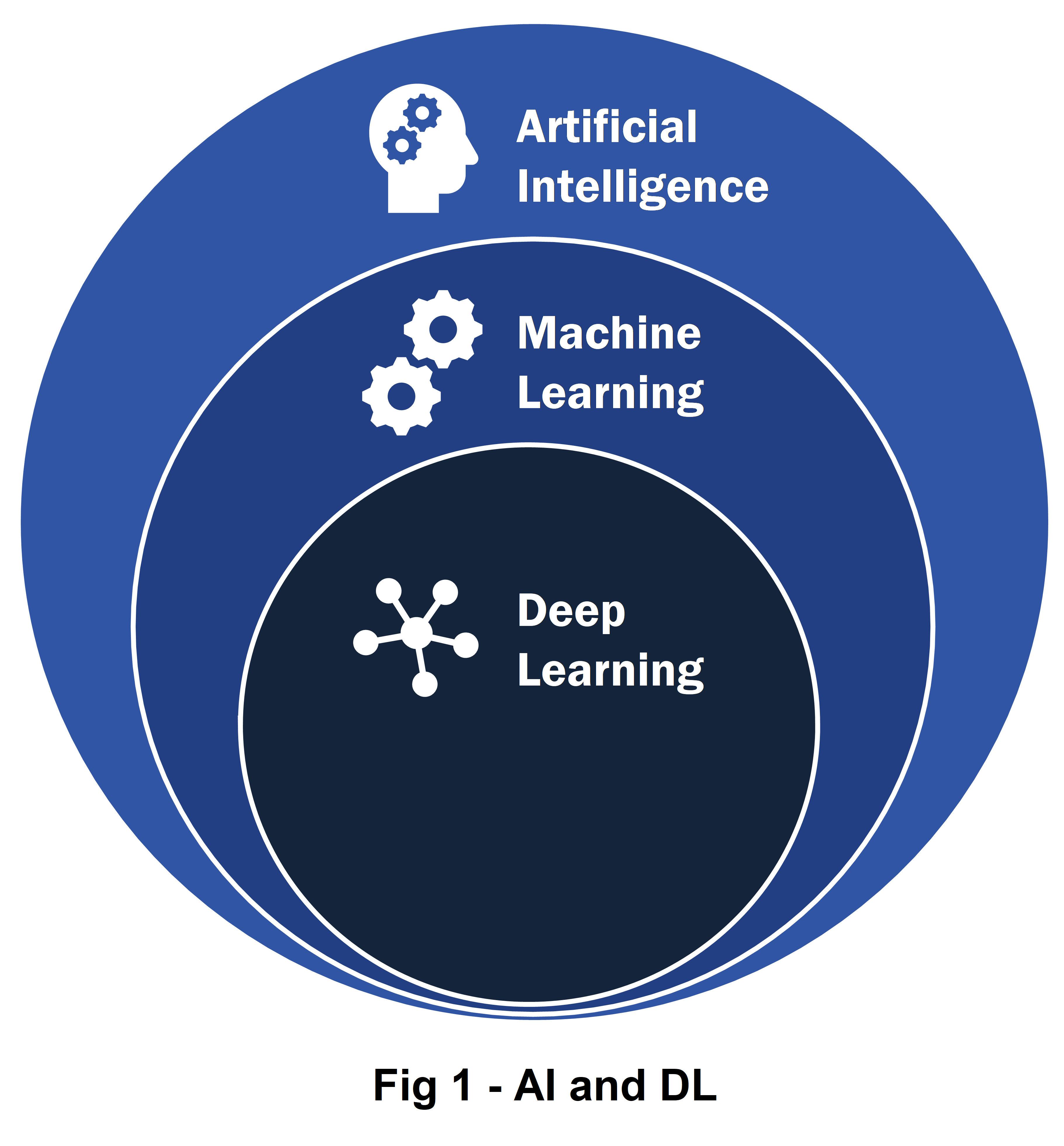
The subset of AI machines is ML which is a series of statistical algorithms and algorithms that programmes a system to perform a specific task without having to code for a “rule-based” instruction set. A powerful example of this is the spam e-mail filtering. Based on a previously existing set of identified spam e-mail addresses, the ML model is programmed to identify specific terms in incoming mail ID to redirect these to the spam folder. This is, of course, not entirely robust as is known from the experience of “please check in your spam folder”.

The last subset³ is deep learning (DL) models and we will be employing these. DL systems identify patterns and cues from multidimensional data structures⁴ without any pre-existing notion of pattern provided. All you tell the DL system, in some sense, is what you expect as the output and what you provide it as input. Some common examples of DL are speech recognition, self-driving cars, portfolio management and stock price movement predictions.

DL machines are some of the most widely used AI systems primarily since they are capable of detecting patterns between variables which might not even be empirically visible as a direct causality. They are capable, at least in theory, of detecting patterns emerging from multiple removed causality correlations. If $x_1$ influences $x_2$ which influences $x_3$, and so on till $x_n$, then a DL model is capable of resolving, to great deal of accuracy, the causality influence of $x_1$ on $x_n$. This is a simple example but in reality, things are more complicated and a DL system is capable of distinguishing patterns there as well. One such sector is the financial stock market sector. The stock market is buffeted by elements that are often simply absorbed into stochastic modelling (as a Brownian motion, perhaps). Patterns might exist between obvious elements, but there is a limit to which conventional modelling of the prices can take into account various factors, primarily owing to the high dimensional nature of the analysis.

VAR models have often been used to computationally model stock prices⁵ but have their limitations which arise from the high dimensional nature of the data. High dimensional data increases the number of parameters that need to be estimated by the VAR which increases the complexity of computation. Assuming a $p$-lag, $k$ variables, the generic VAR model estimates $(k^2 p + k)$ parameters. As you can see, the parameters increase quadratically with respect to the number of variables. The more the number of parameters, the lower the degree of freedom⁶ of the model which drastically affects the accuracy and subsequently the forecasts of the model. Apart from this, there are the obvious assumptions of stationarity and uncorrelated error terms. DL models are free of all these issues. No assumptions have to be made. No limitations are placed. Without going into the mathematics behind the model we will be using, I will introduce the architecture involved to give you a better idea of what happens inside the model. The DL model we will be employing is a modification of the Recurrent Neural Networks (RNN). Let us first understand RNNs.

Humans have persistence of thought – as you read these words, your brain does not (hopefully) have to relearn the alphabets, grammatical structures, and basic semantics to understand each paragraph. Instead, you understand based on your previous recollection of words. When you start reading a new paragraph, your brain does not discard previously stored information (about words and such) to start from scratch. In other words, there is a systematic retentivity that your neurons possess. Traditional ML and DL architectures, such as ANNs, CNNs are incapable of such persistence and retention⁷. For instance, if one wishes to categorize the objects in a live video stream using a DL model, the traditional architecture will have to run over an over again for each frame in the movie (which would take ages). This would make it rather unsafe and, not to mention, impractical to implement in self-driving cars.

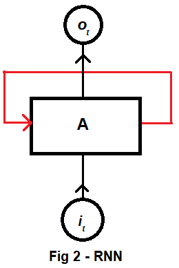
RNNs address this issue by having a loop in the architecture allowing information to persist within the network. Fig 2 shows a diagram for a RNN neuron. $i_t$ is some input at time t with the corresponding output being $o_t$. The red loop allows information to be passed from one time step to another. A RNN is simply a rolled up neural network and are, thus, the natural choice for series and sequence data structures (such as our problem in consideration)⁸ . These RNNs have been extremely successful in the field of DL and are almost the explicit contents of self-driving cars and speech recognition software. But that is a half true statement. The entre truth is that a modification of the RNN is used. This modification itself arose from an issue with the RNN – long term dependencies. In very brief terms, this is an issue arising from the inability of a plain vanilla RNN to connect information from various sources. For example, the stock price might be forecasted using only its own history. This, a plain vanilla RNN can do. But when it comes to finding the pattern that spreads out into various other factors such as, say the price of another parallel stock, or a recent shock in monetary policies, or a natural disaster that triggers CAT swap defaults, in such cases, the plain vanilla RNN fails. To overcome this issue, the Long Short Term Memory networks (LSTMs) were introduced⁹.

I side-step the technicalities of the LSTM to retain readability (something I fear I might have already lost). However, it is imperative that I mention that the LSTM itself does not add or remove data from the neural layer. That ‘authority’ is reserved for the parent RNN structure. There is sufficient literature available on LSTMs which the interested reader can read for further insight.

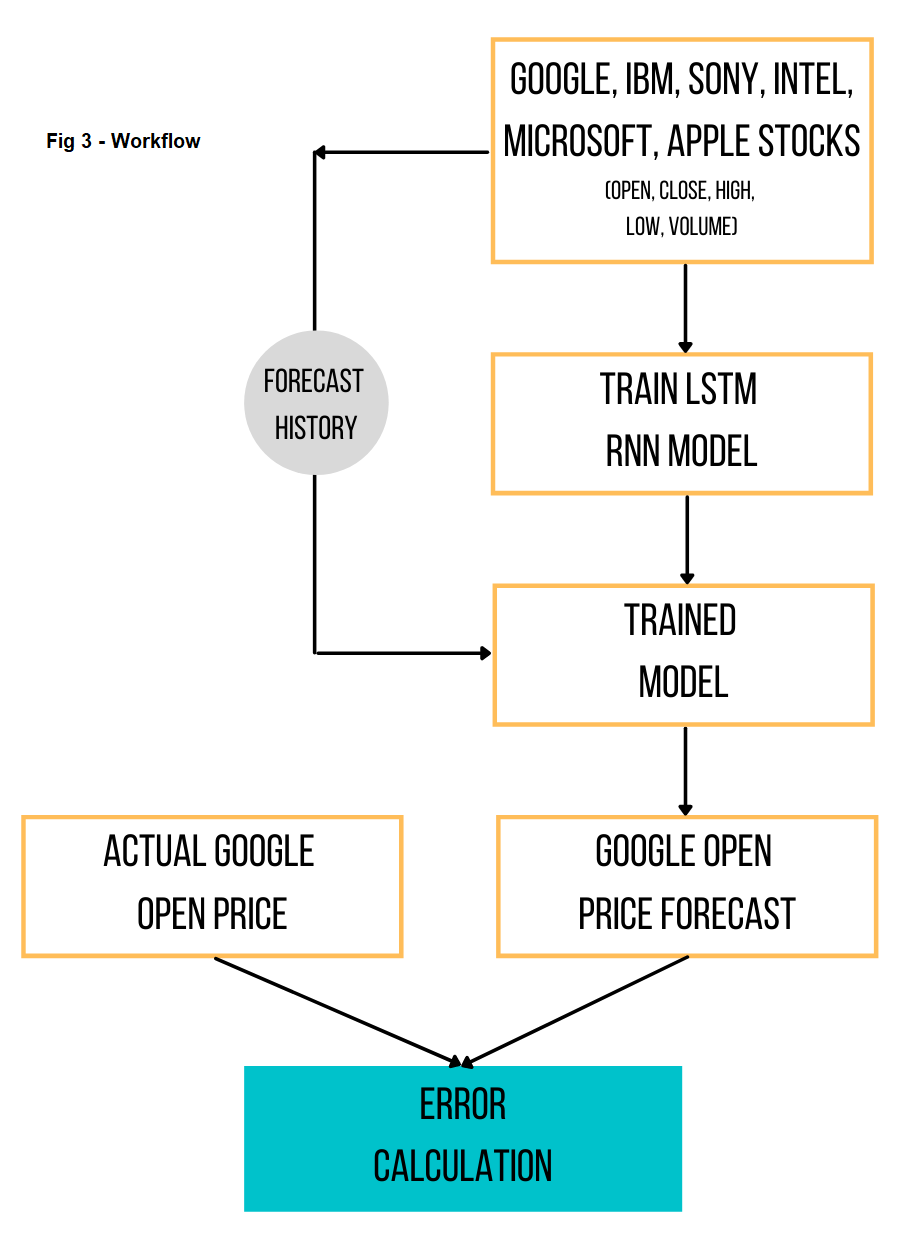
After having laid the foundation of the idea behind the model, let us now take a look at the problem closely. The workflow of the problem is depicted in Fig 3. We attempt to forecast (or predict) the opening price of google on a daily-basis¹⁰. The input for this is the data of open, close, high, low, Adjusted Close, and volume of share prices of the following companies from 19-AUG-2004 to 29-APR-2021.

1. Alphabet Inc (Google)
2. IBM
3. Intel
4. Microsoft
5. Apple
6. Sony

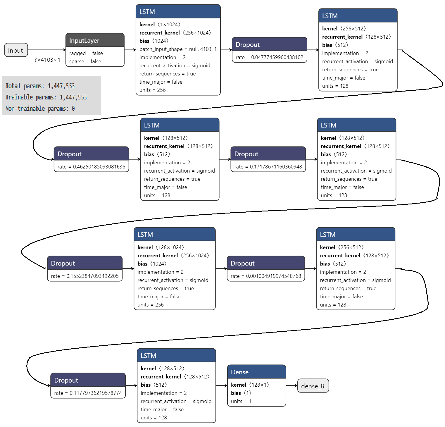
In theory (and in practice) this can be extended to contain all possible stocks and shares as one wishes to in addition to other factors that one may find relevant to the google stock, for example some form of dummy indexes for taxes, or the interest rates. I chose these primarily due to the obvious relation between these companies. All of them are tech giants. The argument is straightforward, an increase in the shares of Microsoft and Intel signals an increase (possibly) in the number of laptops that can use a browser to access google products. I assumed that Apple and Sony might have negative and positive contributions respectively due to the former being a competitor (iOS, iPhones vis-à-vis android etc) and the latter producing mobile phones that run on android. While I made these assumptions, I reiterate that no assumptions need to be made in practice for DL models. One the data-set was ready, it was fed into an LSTM modelled on Keras with a TensorFlow backend. These are Python (a programming language like R) libraries specifically made for ML and DL modelling. The model trains on the dataset barring the latest 40 dates (i.e. 03-MAR-2021 onwards) which we retain for the final testing¹¹. The architecture of the model is given in the figure below.

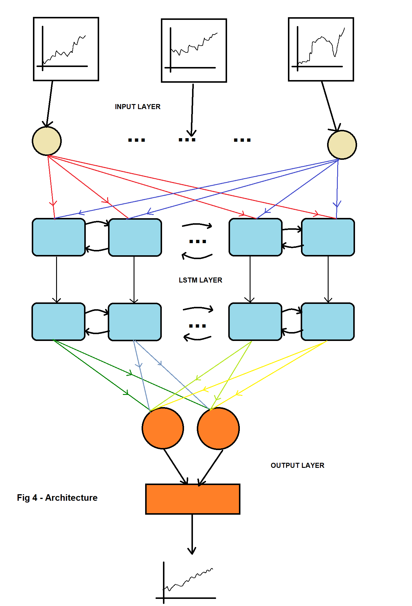
The model was trained for 100 epochs (DL term for steps) on a batch size of 32 on 7 layers of LSTM with dropout¹². The data is initially pre-processed by normalisation. The standard procedure is to use mean squared error to minimise the loss of the model. However, I have used the Huber loss since it is less sensitive to outliers¹³, which in the case of stocks are a-plenty.

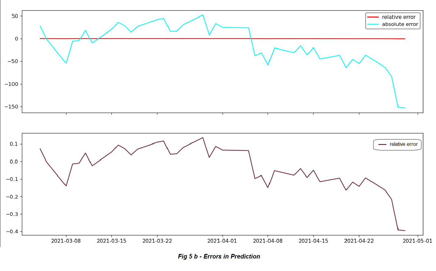
After the model has been trained, we use a ‘lag’ of 60 days¹⁴ to forecast for 40 days ahead. The results were plotted after reverse transforming (from normalisation) are provided in Fig 5 with the errors. The error increases with the increase in the forecast horizon since the errors ‘add up’. As the model estimates the forecast of time $t+1$ from $t$. Then at $t+2$ it uses the forecast from $t+1$. This goes on and the errors simply add up. The schematic of the trained model was exported using Netron (a DL architecture printing software) and is shown in the figure below. The total trainable parameters¹⁵ are 1,447,553.

The output closely resembles, if not entirely, the actual google open stock prices. This is a powerful practical example of the possibility of use of DL in finances. The best part, is that one doesn’t need to know much about neither finance nor the mathematics behind neural networks to implement a marketable model.

✍︎

The author

Vivin Vinod is a postgraduate of Economics from the University of Pisa, Italy. He enjoys poetry and woodwork amongst other co-scholastic things. He is currently involved in researching the applications of machine learning in assisting sign language interpretation. He can be contacted at his .